In the next section for B1705 we’ll explore the topic of ‘time-series analysis’ (TSA).
Time series analysis is essential in understanding how data points collected over time can reveal underlying trends, patterns, and anomalies. Over the next two weeks, we’ll review the tools and techniques essential for decomposing series, detecting seasonality, and understanding the impact of time in data analysis.
47.2 What is time-series analysis?
Time-series analysis (TSA) involves examining data points collected sequentiallyovertime to uncover patterns and trends, and to make future predictions.
In TSA, data is collected in a time-ordered sequence. In sport, this could be daily training metrics, weekly performance data, or seasonal injury records. The key characteristic is that these data points are dependent on time.
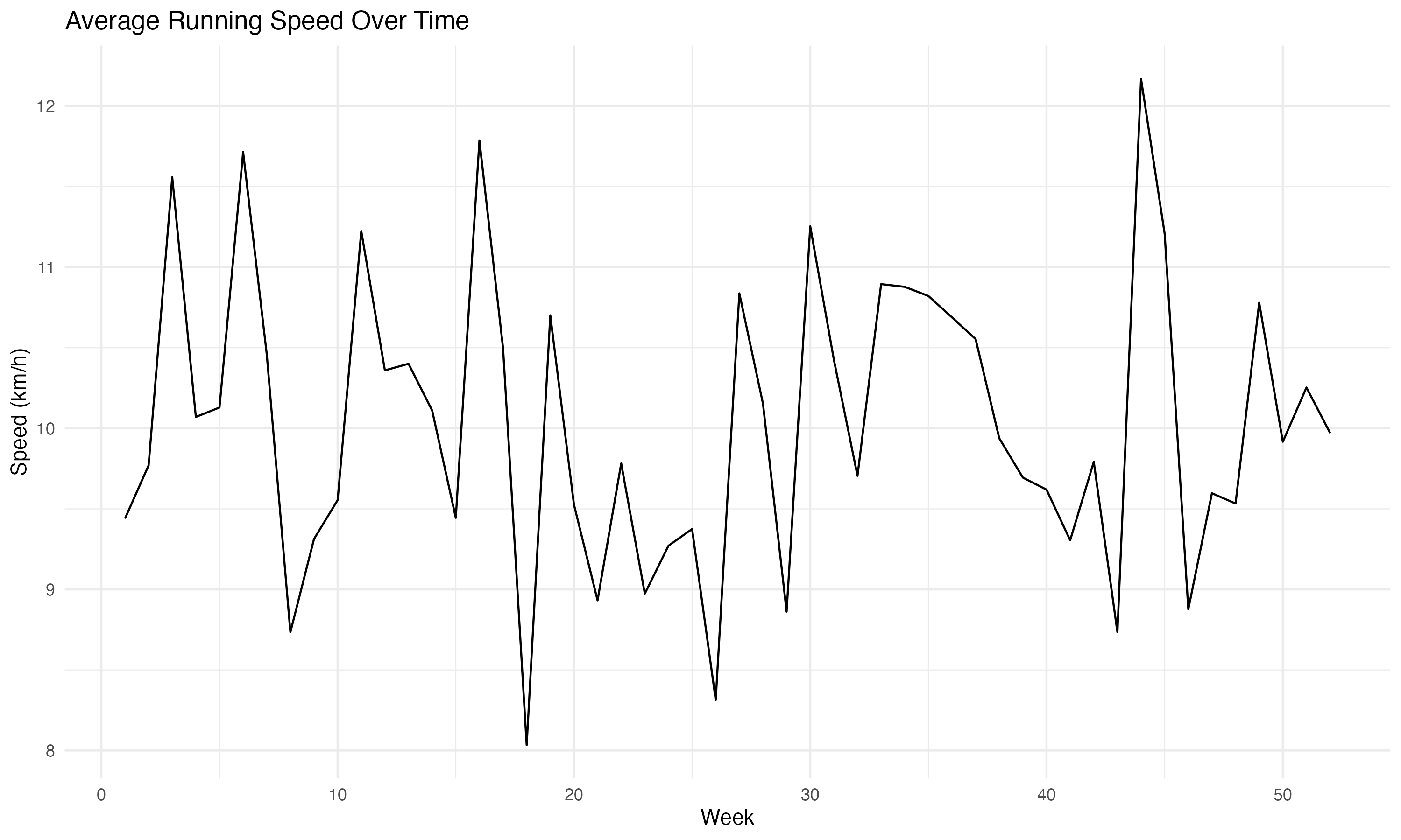
Here’s an example of a time-series, where average weekly speed has been collected over a period of a year.
TSA is based on identifying trends and patterns.
Trends show the general direction of data over time, like a gradual increase in an athlete’s stamina.
Patterns, such as seasonality, reveal regular fluctuations, like performance variations across different seasons or competitions.
Often, TSA is used to forecast future values based on historical data.
Methods that we’ll learn about - like ARIMA (Autoregressive Integrated Moving Average) - can be used to (for example) predict future performance, injury risks, or training outcomes, helping in planning and decision-making.
Applications
TSA is important for several reasons:
it helps in identifying underlying trends and patterns in data collected over time. For sport analysts, this might mean tracking an athlete’s performance or physical condition, allowing us to see improvements, declines, or seasonal variations.
it’s valuable for making informed predictions about future events based on past data. For example, predicting future performance levels, injury risks, or the impact of training regimes on athletes.
by understanding past trends and forecasting future ones, we can help coaches and managers plan more effectively. For example, our analysis might influence optimising training schedules, injury prevention strategies, and competitive readiness.
it can reveal correlations and causal relationships between different variables over time. This helps us understand how various factors like training intensity, diet, and rest impact an athlete’s performance.
it allows for the assessment of the impact of changes or interventions. For example, analysing how a new training method or technology affects an athlete’s performance over time.
47.3 Why time matters
Thinking about time in data is really important, though (in my opinion) very often overlooked in sport data analytics. Ignoring the fact that data is a time-series can lead to several significant issues and risks:
Misinterpretation of data: Without acknowledging the time-dependent nature of data, you might draw incorrect conclusions. For example, in sports science, ignoring time-series can lead to misjudging an athlete’s performance improvement or decline.
Inaccurate predictions: TSA often involves forecasting future values based on past trends. Ignoring the sequential nature of data can result in unreliable and inaccurate predictions, leading to poor decision-making.
Overlooking seasonality and trends: Many datasets in sport exhibit seasonal patterns or trends over time. Ignoring these elements can cause a failure to recognise important cyclical behaviors, such as seasonal peaks in athlete performances.
Failure to identify causal relationships: Time-series data can help in identifying causal relationships. Ignoring the time aspect might lead to overlooking these relationships, potentially leading to ineffective strategies or interventions.
Statistical analysis errors: Many statistical tests assume independence of observations. Applying these tests without considering the time component can lead to erroneous statistical inferences.
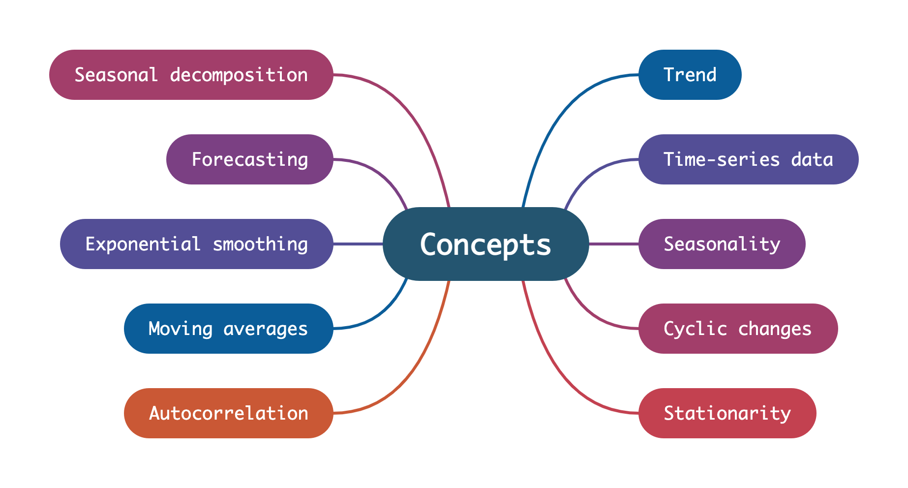
47.4 Key concepts
There are some key concepts that you should grasp before embarking on TSA. We’ll introduce these in the practical this week and they’ll appear throughout this part of the module.
47.4.1 Time-series data
‘Time-series’ data is a sequence of data points collected at consistent intervals over time.
It’s like a diary that records specific measurements, like temperature or stock prices, at regular times. The interval of recording doesn’t matter (second, minute, hour, day); it’s the consistency of recording over time that matters.
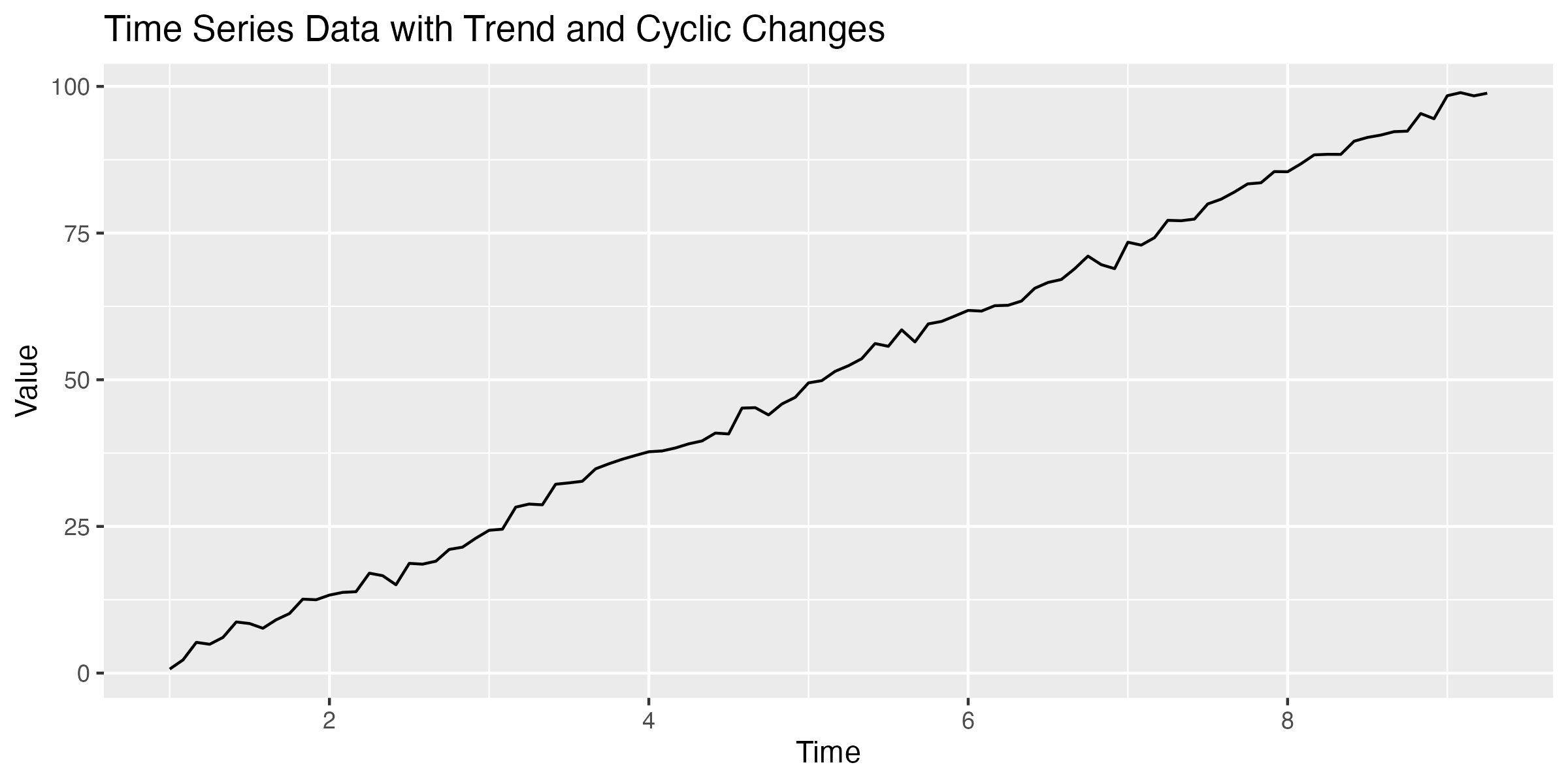
47.4.2 Trend
In time-series data, a ‘trend’ is the overall direction in which the data is moving over time. It can go up, down, or stay relatively flat.
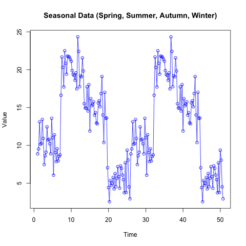
47.4.3 Seasonality
‘Seasonality’ refers to regular, predictable changes that occur in time series data at specific periods, much like the way ice cream sales increase in summer and decrease in winter.
47.4.4 Cyclic changes
‘Cyclic changes’ are long-term fluctuations in time-series data without a fixed pattern, similar to economic booms and recessions, which don’t follow a strict schedule but happen every few years.
47.4.5 Stationarity
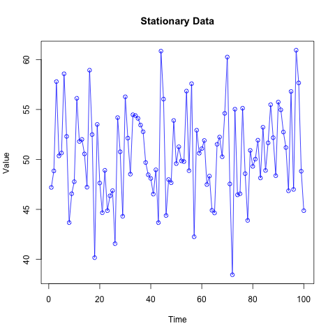
A time-series is ‘stationary’ if its statistical properties, like mean and variance, remain constant over time. It’s like a calm sea where the overall water level doesn’t rise or fall dramatically over time (see the first figure below).
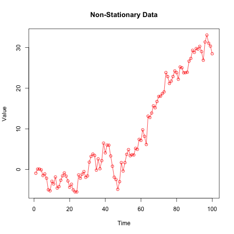
‘Non-stationary’ data, on the other hand, has a clear trend (shown in the second figure) so the mean and variance change over time.
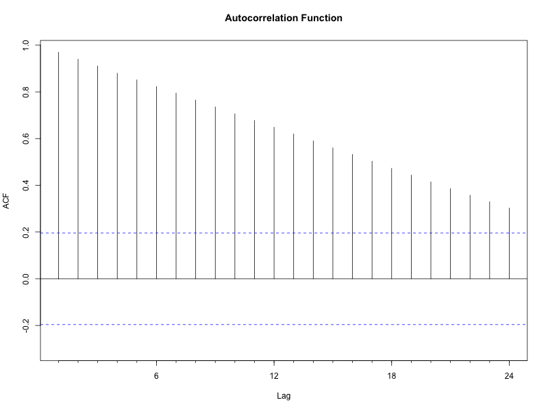
47.4.6 Autocorrelation
Autocorrelation is when a time-series is correlated with itself at previous times.
You might assume that how much coffee you drink today is related to how much you drank yesterday. Or if you’re on campus every Wednesday, your coffee consumption each Wednesday is likely correlated to how much you drank last Wednesday.
For athletes, it’s likely that their performance today is related to how they performed yesterday. This is an example of autocorrelation.
47.4.7 Moving averages
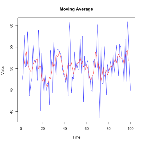
Moving averages smooth out short-term fluctuations in time-series data to identify longer-term trends, like averaging your daily steps over a week to understand your general activity level.
In the following figure, the raw data is in blue and the moving average is in red.
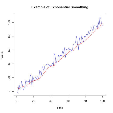
47.4.8 Exponential smoothing
This technique gives more weight to recent observations while smoothing time series data, like a weighted average where recent team scores matter more than older ones.
In the following figure, the data is in blue and the exponential smoothing is in red.
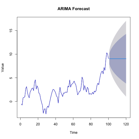
47.4.9 Forecasting
Forecasting in time-series analysis means predicting future data points based on past trends, like using past weather patterns to forecast tomorrow’s weather.
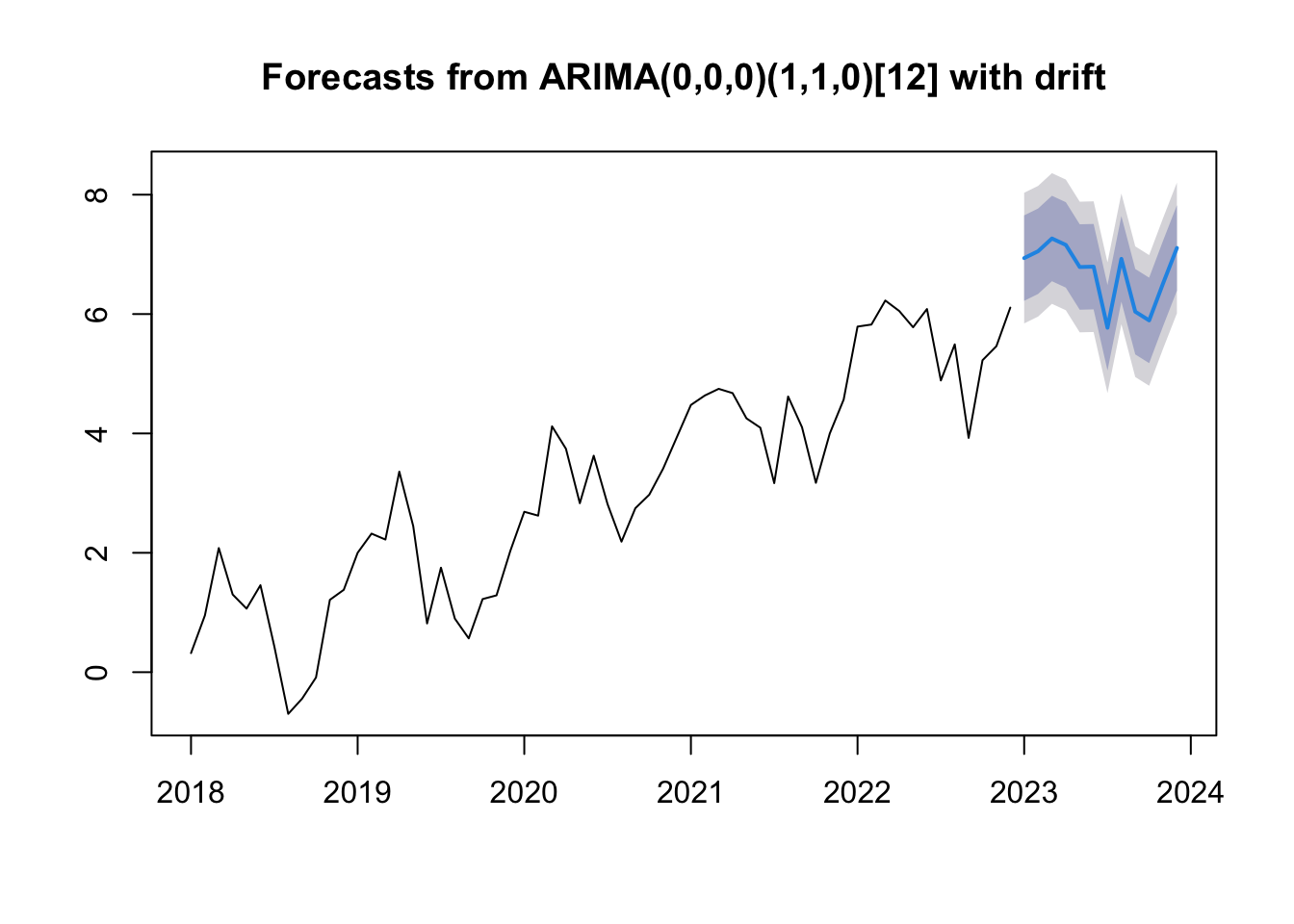
For example, one model we often use is ARIMA (Autoregressive Integrated Moving Average):
ARIMA is a complex forecasting method for time series data that combines trends, seasonality, and other factors to predict future points.
Here’s an example where the existing data is shown in blue, and the forecast can be seen at the far right:
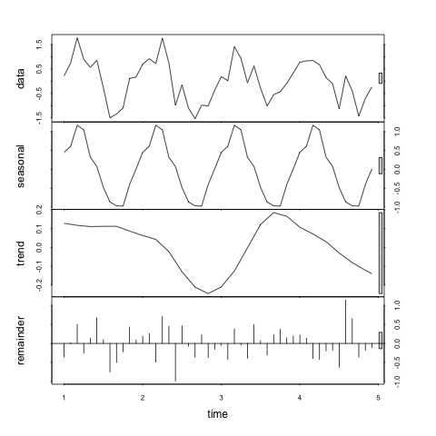
47.4.10 Seasonal decomposition
Seasonal decomposition breaks down time-series data into trend, seasonal, and random components, like dissecting how much of a team’s performance is due to time of year, general trends in its performance, or random/unexpected events.
In the second row of this plot, note how there is a clear seasonal effect in the data (note: ‘seasonal’ doesn’t mean the seasons of the year, though these can be an example of this effect).
47.5 TSA in R
Now, we’ll briefly review how to approach TSA in R.
This will be covered in much more depth in the practical session this week. This is just intended as a basic introduction to time series in R.
Step One: We load the data into a dataframe data
Load and inspect data
data <-read.csv('https://www.dropbox.com/scl/fi/755z2zrppejfazkun5h7t/tsa_01.csv?rlkey=e5welqld5idyeb0ccwa44whfj&dl=1')head(data)
  X       Date     Value
1 1 2018-01-01 0.3197622
2 2 2018-02-01 0.9509367
3 3 2018-03-01 2.0793542
4 4 2018-04-01 1.3012796
5 5 2018-05-01 1.0646439
6 6 2018-06-01 1.4575325
Step Two: Convert the data to a time series object ts_data
R needs to be told that our data is in the form of a time-series.
We have to convert it in order to use the time series functions. ts is often used for this purpose.
Show code
# Convert the data to a time series object called ts_datats_data <-ts(data$Value, start =c(2018, 1), frequency =12)
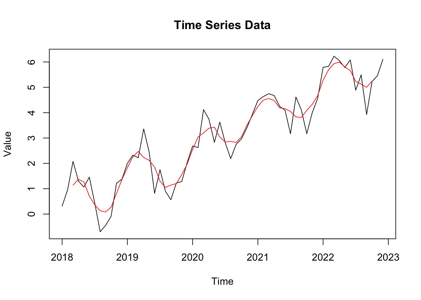
Step Three: Plot the data and apply a simple moving average
We can now visually inspect our time series data. The moving average shows the general pattern within our data.
Show code
# Plot the time series dataplot(ts_data, main="Time Series Data", xlab="Time", ylab="Value")# Apply a simple moving averagelibrary(stats)moving_avg <-filter(ts_data, rep(1/5, 5), sides =2)lines(moving_avg, col="red")
Step Four: Use ARIMA to forecast the future
Time series analysis is often used to forecast what might happen in the future. We can use R to do this, for example by using the ARIMA model:
Show code
# Forecasting using ARIMAlibrary(forecast)arima_model <-auto.arima(ts_data)forecasted_data <-forecast(arima_model, h=12) # forecast for the next year# Plot the forecastplot(forecasted_data)
47.6 Conclusion
Hopefully, this section has provided you with an introduction to the basic tools and concepts that we will continue to explore throughout our exploration of time-series analysis.